
Artificial Intelligence Algorithms
- Artificial intelligence can be used to automatically create models from data.
- Typically not guaranteed to find perfect models, but may be able to find good models, depending on the difficulty of the problem and on the data available.
- Good for problems where there is no need for a perfect model.
- Good for problems where models are necessary and it is difficult to create good models manually.
Logics
- Knowledge is represented in the form of logical statements.
- New knowledge can be inferred from existing statements.
- Problems can be solved based on such knowledge.
Definitions
Many different definitions, such as think humanly, act humanly, think rationally, act rationally.
We will adopt Russell and Norvig’s definition:
Artificial Intelligence is the area of Computer Science which studies rational agents.
Rational agents are computer programs that perceive their environment and take actions that maximize their chances of achieving the best [expected] outcome.
Breadth-First and Depth-First Search
1. Problem Solving Agent
- Agents may need to be able to plan ahead, i.e. to reason so as to find a sequence of actions needed to solve a task.
- Problem-solving agents are agents able to search for a solution to a given problem.
2. Problem Formulation
- A problem formulation is necessary so that the agent knows what problem needs to be solved.
- Elements of a problem formulation:
- Initial state.
- Goal state(s).
- Possible actions and their effects on states.
- Cost function.
Example
- Initial state & Goal state.
- Possible actions (Using State Space Graph, SSG Notation: represent states, you will need to decide on a good representation for the states, so that the implementation of the algorithm is efficient)
- Uninformed Search Algorithms
- Search trees & notation
- Cost
3. Uninformed Search Algorithms
- Search algorithms search for solutions to a given problem.
- Input: problem formulation.
- Output: solution, in the form of a sequence of actions.
- Once the solution is known, its actions can be carried out.
- Uninformed search algorithms have no information about states beyond that provided in the problem definition.
4. Search Trees
A search tree can be generated to search for a solution. Each node corresponds to a state and has a single parent. Each edge corresponds to an action applied to a state.
The tree represents only the explored portion (or less) of the graph as a search tree. The state space graph could be very big, even could be infinite large.
If a state can be reached by two nodes, we only remember the node associated to the lowest cost. We always want the cheaper solutions.
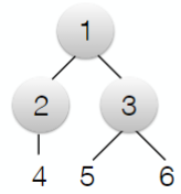
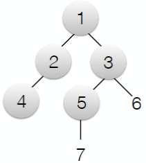
Search Trees: 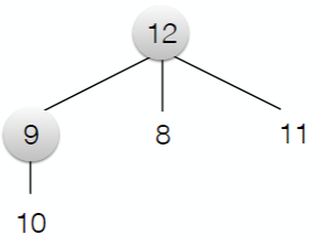
When we try to expand a node, we will mark it by a circle. We say that this node has been visited. The set of nodes in the tree that are available to be expanded are called the frontier.
Different search techniques essentially correspond to different ways of deciding the next frontier node to visit. Breadth-first and depth-first search are techniques that can be used when the cost of each action is 1.
5. Breadth-First Search
1. Algorithm
- Visit the shallowest frontier node first, placing its children in the frontier.
- Do not place children in the frontier if their corresponding state is already in the frontier or list of visited nodes.
- Stop when you place in the frontier a node which is a goal node.
2. BFS as a First In First Out (FIFO) Algorithm
The frontier can be seen as a FIFO queue. The element that was queued first is the first one to be visited.
3. Properties
Branching factor: b , the branching factor is the master of children at each node.
Depth of the shallowest goal state: d
- Complete: so long as b is finite, it is guaranteed to find a path to a goal state if on exists, or to terminate in failure.
- Optimal: guaranteed to find the shortest path to a goal state first (when all actions have the same cost).
- Memory complexity:
. - Time complexity:
.
6. Depth-First Search
1. Algorithm
- Visit the deepest frontier node first, placing its children in the frontier.
- Do not place children in the frontier if their corresponding state is already in the frontier or list of visited nodes.
- Stop when you visit a node which is a goal node.
2. DFS as a Last In First Out Algorithm
We can see the frontier as a LIFO queue (stack). The element that was piled last is the first one to be visited.
3. Properties
- Complete if the state space is finite: it is guaranteed to find a path to a goal state or to terminate in failure.
- Not complete if the state space is infinite.
- Not optimal: not guaranteed to find the shortest path to a goal state first.
- Memory complexity:
.
4. Saving Space Complexity
- The version of depth-first search shown in the previous slides needs to store all previous visited states.
- If we store only the nodes in the path from the root to the current node, we could save space, while still being complete for finite state spaces.
- Space complexity:
. - Time complexity:
. - Where b is the branching factor and m is the maximum depth of the search tree.
- Space complexity:
7. Depth-Limited Search
- To guarantee that depth-first search will terminate (either in success or failure) in a reasonable amount of time, we can put a limit on the maximum search depth.
- If the goal's depth d<=L then depth-first search is complete.
- Still not guaranteed to find the shortest path (i.e. not optimal).
- Depth limited search performs depth-first search to a depth limit L.
- Time complexity
. - Space complexity
.
- Time complexity
8. Analyzing Search Algorithms
- Completeness — A search algorithm is complete if it is guaranteed to find a solution when at least one solution exists.
- Optimality — A search algorithm is optimal if it is guaranteed to find the best solution when there is more than one solution (sometimes termed optimality)
- Time Complexity — The order of computation required during the search process to find a solution in the worst case.
- Space Complexity — The order of storage space required at any point during the search process in order to find a solution in the worst case.
Other
1. Cost
Cost of the solution = sum of the costs of the actions
2. State Space Graph
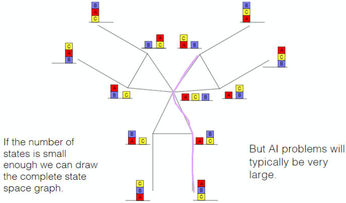
A solution can be seen as a path in the state space graph.