
Hash tables & Graphic
Hash Tables
1. Summary
A hash table consists of
- an array
arrfor storing the values. - a hash function
hash(key). - a mechanism for dealing with collisions.
Basic operations
put(key, value)delete(key)get(key)
Disclaimer: We will consider a simplified situation where keys and values are the same. For example, an assignment is always:
arr[hash(key)] = key.
2. Two types of solutions of hash collisions
1. Sticking out strategy
2. Tucked in strategy
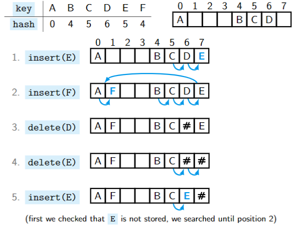
Linear Probing
Insertion (initial idea): If the primary position
hash(key)is occupied, search for the first available position to the right of it. If we reach the end, we wrap around.Deletion:
Find whether the
keyis stored in the table: Starting from the primary positionhash(key), go the right, until thekeyor an empty position is found.If the
keyis stored in the table, replace it with a tombstone (marked as #).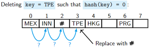
Searching:
Starting from the primary position
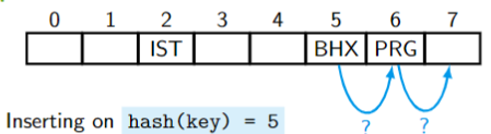
hash(key), search for thekeyto the right. We skip over all tombstones #. If we reach an empty position, the thekeyis not in the table.Inserting (more accurately):
- check if
keyis stored in the table , and - if it is not and its the primary position
hash(key)is occupied by a different key, search for the first empty or tombstone position to the right of it. - Store the
keythere.
- check if
Double hashing
To deal with the problem caused by Primary clusters, we need to use double hashing.
Use primary and secondary hash functions hash1(key) and hash2(key), respectively.
Insertion: We try the primary position
hash1(key)first and, if it fails, we try fallback positions:(hash1(key) + i*hash2(key)) % TABLE_SIZE(until we find an available space).
Avoiding short cycles
- T is a prime number.
and hash2(key)is always an odd number. (preferred)
3. Time Complexity
The load factor of a hash table is the average number of entries stored on a location:
n = the total number of stored entries, T = the size of the hash table. If we have a good hash function, a location given by hash(key) hash the expected number of entries stored there equal to
3. What to do if the table is full?
We say that a hash table is full if the load factor is more than the maximal load factor, that is,
Rehashing (idea): If the table becomes full after an insertion, allocate a new twice as big table and insert all elements from the old table into it.
Graphs and graph algorithms
A graph is formed of a (finite) set of vertices/nodes and a set of edges between them. We distinguish four types of graphs: 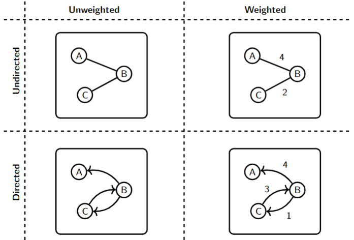
1. Adjacency Matrix
Assume that graph's vertices are numbered
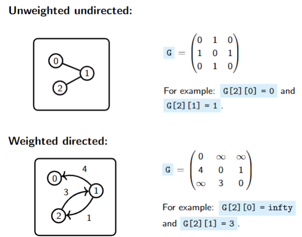
Adjacency matrix G is a two-dimensional array/matrix
- Unweighted graphs:
G[v][w]= 1 if there is an edge going fromvtowG[v][w]= 0 if there is no such edge
- Weighted graphs:
G[v][w]= weight of the edge going fromvtowG[v][w]=if there is no such edge G[v][w]= 0
- Remark: The graph is undirected if
G[v][w] = G[w][v]for all verticesvandw.
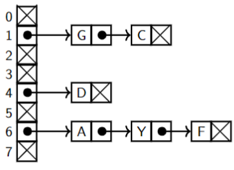
2. Adjacency List
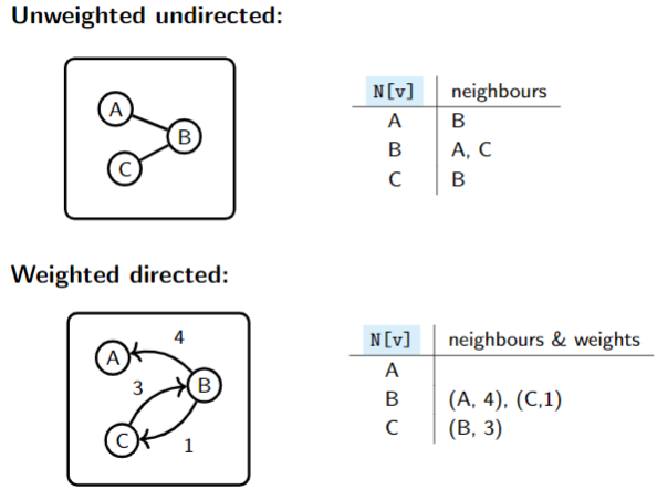
To represent a graph on vertices N of n-many linked lists (one list for every vertex).
- Unweighted:
N[v]is the list of neighbors ofv. (wis a neighbor ofvif there is an edge)
- Weighted directed:
N[v]is the list of neighbors ofvtogether with the weight of the edge that connects them withv.
For example,
N[2]stores the address of the head of the linked list of all neighbors of the2nd vertex.
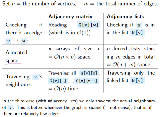
3. Comparison
4. Paths and shortest paths
1. Definition
A path from v to z is a sequence of edges v with z.
The shortest path is the path such that the sum of weights of its edges is the minimal. (In unweighted graphs, set weights to 1.)
2. Dijkstra's algorithm
View Youtube.
3. Prim's algorithm
View Youtube.